Introduction
Insertion sort is a simple and useful sorting method. In this article I’ll explain insertion sort time complexity in plain words. You will learn when it runs fast and when it runs slow. I will show examples, clear rules, and real tips you can use. I wrote this to be easy to read. Sentences are short and clear. I also add small stories and code ideas to build trust. By the end you will know how insertion sort behaves, why that behavior happens, and when to choose it. You will also get answers to common questions. Let’s get started and make sorting feel natural and useful.
What is insertion sort?
Insertion sort is a way to sort items by building a sorted list one item at a time. You take each new item and place it in the right spot. You shift larger items to the right to make space. This method is like sorting playing cards in your hand. You look at one card and slide it into the right place. The algorithm works in place, so it needs little extra memory. It compares and moves items until the entire list is sorted. In small lists, insertion sort often beats more complex algorithms. The logic is simple, and the code is short. That simplicity makes it a great teaching tool and a practical choice in some real programs.
How insertion sort works — step by step
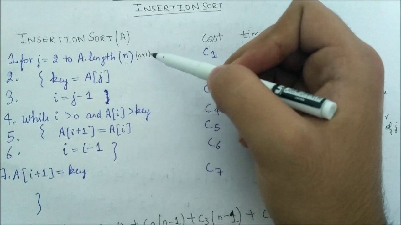
Imagine you have a list of numbers on paper. Start at the second number. Compare it with the numbers to its left. Move leftward until you find where it fits. Shift each larger number one spot to the right. Insert the item at the empty spot you made. Repeat this for every item until the list is sorted. Each pass grows the left part of the list that is already sorted. The right part still needs work. The algorithm uses nested work: an outer loop for each item and an inner loop to find the place. That inner loop does comparisons and shifts. The total work depends on how many times that inner loop runs across the whole list.
Big-O and time complexity overview
When people analyze algorithms, they use Big-O notation to describe time cost. For insertion sort, there are three common cases. Those are best, average, and worst. Each case gives a different Big-O. The best case happens for nearly sorted input. The worst case happens for reverse order input. The average case is what you expect for random lists. In simple words, insertion sort time complexity varies with the input order. That variation is key to understanding when the sort is a good pick. Below we break down each case and show how many comparisons and shifts to expect.
Best-case time complexity: O(n)
The best case for insertion sort is when the list is already sorted. In that situation, every new item only needs one comparison. The inner loop finds the spot immediately. There are no shifts to move larger items. So the outer loop runs n−1 times and the inner step runs once each time. That gives a linear cost, O(n). This makes insertion sort adaptive. When input is already nearly sorted, it runs very fast. That property is useful for some real tasks, like refining nearly sorted data or merging small sorted runs. If your data tends to be ordered, insertion sort time complexity is very attractive.
Average-case time complexity: O(n²)
For random input, insertion sort usually needs to shift items a lot. On average each new item moves about half the way left. That means the inner loop does about n/2 checks per item on average. Multiplying across n items gives a quadratic cost. So the average time is O(n²). In practice this makes insertion sort slow on medium to large lists. It is okay for lists of tens or low hundreds of items. But for big data sets, the quadratic growth becomes too slow. Still, the simplicity and small memory use can make insertion sort useful inside other algorithms or for short runs inside hybrid sorts.
Worst-case time complexity: O(n²)
The worst case happens when the list is in reverse order. Every new item must go all the way to the front. That forces the inner loop to do the maximum work each time. So the total number of comparisons and shifts is on the order of n². This is the same Big-O bound as the average case, but now constants are larger. The performance degrades quickly as n grows. For this reason, insertion sort is not a good choice for large, unsorted data where worst-case scenarios are common. Still, knowing the worst case helps plan when to switch to faster algorithms like mergesort or quicksort.
Space complexity and stability
Insertion sort works in place. It uses only O(1) extra memory on top of the input. That is, it needs a small number of extra variables. This makes it memory friendly. Another good property is stability. Items that compare equal keep their original order after sorting. Stability matters when sorting complex records by one key while keeping other keys’ order. The low space cost and stability are reasons programmers sometimes pick insertion sort for small tasks. When memory is tight or stability matters, insertion sort is a solid, simple choice.
Why insertion sort is adaptive and online
Insertion sort is adaptive because its running time improves for inputs that are already close to sorted. The more ordered the input, the less work the algorithm must do. It is also an online algorithm. That means it can sort items as they arrive, one by one. You do not need the full list up front. You can insert new items into the sorted prefix and keep moving. This is useful for streaming data or when you must maintain a sorted list dynamically. Both adaptiveness and online behavior are rare in many simple sorts, which adds value to insertion sort beyond raw speed.
Use cases: when insertion sort shines
Insertion sort shines in several real situations. It is great for tiny lists, where its low overhead beats complex sorts. It is ideal when the list is nearly sorted already. It works well in hybrid algorithms to sort small subarrays after a divide-and-conquer pass. It is also useful in systems with low memory, because it is in place. Insertion sort can maintain a sorted list while data streams in. For teaching, it helps explain core sorting ideas and algorithm analysis. For practical engineering, it is often used inside larger sorting routines as the final cleanup step for small runs.
Implementation example — Python and Java (explanation + short code)
Below I explain a simple implementation and include short code examples. The idea is to walk through one loop that inserts items into a sorted prefix. In Python, you use a for loop and while loop to shift items. In Java, the pattern is similar with for and while loops and array indexing. Both versions require careful handling of the temporary variable you move around. The code is short and clear, typically under a dozen lines for each version. You will see the same core operations: compare, shift right, and insert. These implementations make it easy to test and to measure insertion sort time complexity in practice.
# Python insertion sort (simple)
def insertion_sort(arr):
    for i in range(1, len(arr)):
        key = arr[i]
        j = i - 1
        while j >= 0 and arr[j] > key:
            arr[j + 1] = arr[j]
            j -= 1
        arr[j + 1] = key
// Java insertion sort (simple)
void insertionSort(int[] arr) {
    for (int i = 1; i < arr.length; i++) {
        int key = arr[i];
        int j = i - 1;
        while (j >= 0 && arr[j] > key) {
            arr[j + 1] = arr[j];
            j--;
        }
        arr[j + 1] = key;
    }
}
Optimizations and variations
You can tweak insertion sort in helpful ways. One trick is to use binary search to find the insertion point. This reduces comparisons from O(n) to O(log n), for each insertion. However, shifts still cost O(n), so the overall time remains O(n²). Another idea is to use sentinel values to avoid boundary checks. You can also use insertion sort to merge small sorted runs in hybrid sorts like Timsort. For linked lists, insertion sort can run faster in practice because shifting is cheap. Each optimization can change constants and practical speed, but it cannot change the quadratic worst-case growth for plain arrays.
Comparing insertion sort with other sorting algorithms
Insertion sort shares traits with other simple sorts. Bubble sort is also O(n²) on average, but insertion sort often does fewer swaps. Selection sort has O(n²) time but does fewer writes than insertion sort. Merge sort and quicksort give much better average time, O(n log n), for large n. Quicksort often wins in practice for big arrays, but it needs extra care for worst-case input. Merge sort uses extra memory but guarantees O(n log n) worst case. In short, insertion sort is friendly for small or nearly sorted data, while divide-and-conquer sorts win for large general data. Keep these tradeoffs in mind when you pick a sort.
When not to use insertion sort
Avoid insertion sort for big, random data sets. The quadratic time makes it scale poorly. If you need strict worst-case guarantees with large n, use merge sort or heap sort. If your data is huge and you want low average time, use quicksort or optimized library sorts. Also avoid insertion sort in tight production loops where n varies and can grow. That said, it remains a solid choice inside hybrid sorts or as a final pass for small partitions. Know the data shape and choose a sorting method that matches the playbook.
Measuring and reasoning about time in practice
When you measure insertion sort time complexity in practice, use careful benchmarks. Test with sorted, reverse, and random inputs. Time both comparisons and data moves. Use real-world data samples if you can. Microbenchmarks can mislead if they use unrealistic data shapes. Remember that CPU caches, memory layout, and language implementations affect measured speed. Theoretical Big-O tells growth but not exact wall time. So combine theory with experiments. If you are evaluating an algorithm for production, profile on expected inputs and do the math for n ranges you actually see.
Common mistakes and pitfalls
A common mistake is to assume insertion sort always runs fast. It does not for large random arrays. Another pitfall is forgetting stability when transforming code. Small coding bugs can break the stable order or cause an off-by-one error. People also misuse binary search insertion without handling shifts, which still cost O(n). Finally, using insertion sort blindly inside larger systems without checking typical n can cause slowdowns. The cure is testing, code review, and clear documentation about when the algorithm should be used. These practices keep insertion sort effective and safe in real systems.
My experience and a small story
I once used insertion sort to tidy up a list of timestamps on a device. The list had only 40 items and was nearly sorted. Using insertion sort kept memory low and the code short. It finished instantly. Later I swapped it into a larger system and didn’t test input size. That caused a slow step and a late fix. From that I learned to match the algorithm to expected data size. Use insertion sort for small, tidy jobs, and always test when changing environments. Real experience like this helps me choose the right tool every time.
Conclusion — quick checklist and next steps
Insertion sort is simple, stable, and in place. Its insertion sort time complexity ranges from O(n) in the best case to O(n²) on average and worst case. Use it for small lists, nearly sorted lists, or as a hybrid tool. Avoid it for large random data that needs speed. Test on real inputs and measure time and memory. If you want, try the code examples above and run them on your data. If you need help tuning or picking a sort for a particular system, tell me about your typical data sizes. I’m happy to help you pick and test the right approach.
Frequently Asked Questions
Q1: What is the exact insertion sort time complexity for best, average, and worst cases?
Best case is O(n) when the array is already sorted because each item inserts without shifts. Average case is O(n²) for typical random data because items move halfway on average. Worst case is O(n²) when the input is reverse sorted and each insertion must scan to the front. Remember these Big-O values describe growth with n, not exact clock time. Also consider the number of swaps and comparisons when measuring runtime on real hardware.
Q2: Does insertion sort use extra memory?
Insertion sort is in place and uses O(1) extra memory. You only need a small number of variables for the current item, an index, and temporary storage. This low space usage makes insertion sort useful when memory is limited. If you change the structure, like using a linked list, memory use patterns shift. But the classic array implementation keeps memory cost tiny while still sorting the array directly.
Q3: Can insertion sort be faster than quicksort?
Yes, for small arrays or nearly sorted data, insertion sort can beat quicksort in real wall time. Quicksort has overhead for recursion and partitioning and needs more complex code. For tiny n, that overhead matters. Many practical sorting libraries switch to insertion sort for small partitions to gain this speed. However, for large random data, quicksort typically outperforms insertion sort by a wide margin.
Q4: What is the effect of using binary search with insertion sort?
Using binary search cuts the number of comparisons per insertion from O(n) to O(log n). But you still must shift elements to make room for insertion, which costs O(n). Thus overall time remains O(n²) for array implementations. Binary insertion can reduce comparisons but not the total move cost. It is a useful tweak when comparisons are expensive and moves are cheap.
Q5: Is insertion sort stable and why does stability matter?
Insertion sort is stable in its typical implementation. Equal elements keep their original relative order. Stability matters when sorting by multiple keys in sequence or when you need to preserve secondary ordering. For example, if you sort a list of people by birth month and then by name, stability ensures the earlier order remains intact where keys tie.
Q6: When should I choose insertion sort in production code?
Choose insertion sort when n is small, when data is mostly sorted, or when you must keep memory use minimal. It is also a good candidate for embedded or low-resource environments. In hybrid systems, use it to finish sorting small partitions after a faster divide-and-conquer pass. Always profile on real inputs and include clear comments in the code to explain why insertion sort was chosen.
Leave a Reply